Building an Enrollment Predictor From Noisy ClinicalTrials.gov Data
This project began with a broad request to Sennen: build a model that predicts clinical trial enrollment status after 12 months.
Sennen’s, our CC / Codex plugin, first useful move was not to train a model. It was to push back on the phrasing. “Enrollment status after 12 months” could mean at least four different things, and each of them would produce a different dataset and a different model. That early correction set the tone for the whole project: when the question was vague, Sennen narrowed it; when the data was messy, Sennen surfaced some of the disarray; when an idea sounded promising, Sennen ran it and let the metrics decide.
The result was not one clever architecture. It was a sequence of prompts, experiments, failures, and reframings that gradually turned a fuzzy modeling idea into something credible.
Example 1: Real Data Are Messy
The first concrete step was to have Sennen ingest the ClinicalTrials.gov interventional corpus, flatten it, and get the modeling work started (
/sen:data). That part was straightforward.But ClinicalTrials.gov is more of a noisy administrative registry snapshot, rather than a clean data set. Sennen immediately pointed out mixed precision fields, some records had anchors later than their last updates. Important fields were missing at scale. Some statuses were too administrative to treat as direct operational truth (
/sen:defects).The next step was to visualize the data (
/sen:visualize):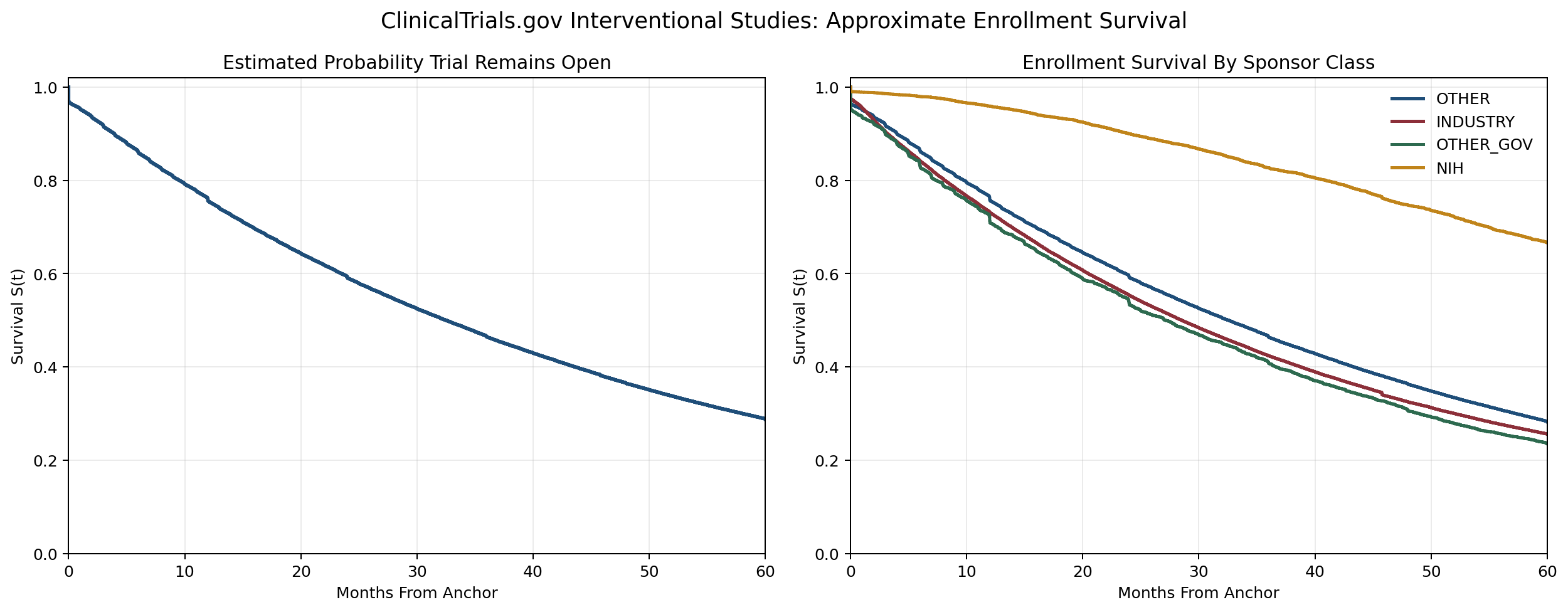
Example 2: The Split Mattered More Than the First Model
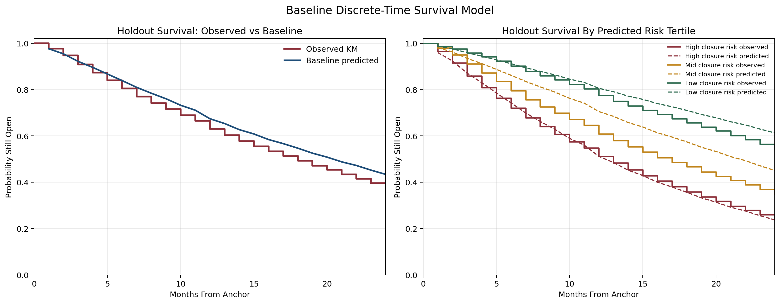
Once the data was loaded and visualized, the natural subsequent step was to build a baseline (
/sen:baseline).Sennen did, but that was not as important as reviewing the split (
/sen:split). Sennen moved the workflow to a temporal holdout and then, after a push for a harder test, added an unseen-sponsor split.That changed the project from “fit a model to historical rows” to “test whether this generalizes to future trials and future sponsors.”
A request for better evaluation turned into concrete split logic, quality filters, and explicit leakage controls. The project became more stringent before it became more accurate.
Example 3: A Simple Sparse Model Beat the Fancy Ideas
Once the task and split were stable enough, the next step was a stronger follow-up experiment (
/sen:experiment again). The first serious winner came from a tuned sparse-text model that used launch-time fields such as title, conditions, interventions, and structured protocol metadata.Then came the usual temptation: maybe embeddings would do better. Maybe a latent representation would do better. Maybe a stacked blend would do better. Sennen ran those paths. Most of them did not improve the metrics.
That failure pattern was genuinely useful. It showed that for registry text, direct sparse representations were stronger than compact generic sentence embeddings (at least for the models tried).
Example 4: Cleaning the Data Changed the Story
One of the less glamorous but most consequential turns came from asking Sennen to inspect defects in the data itself (
/sen:defects).That review surfaced, as mentioned, exactly the kinds of issues that make registry-derived modeling fragile: future-dated anchors, anchors after last update dates, mixed date precision, and noisy state labels. When ask, the agent built cleaning logic around those defects and reran the experiments (
/sen:preprocess).This was one of the strongest “don’t skip the boring part” moments in the project. Some experiment branches that looked unstable or unimpressive before cleaning became much stronger afterward.
Example 5: Better Features Helped, But Not in the Expected Way
Once the sparse-text baseline had become more credible, the next question was what else could be added.
That led to work on therapeutic area, modality, targets, and external scientific data (
/sen:data). Sennen responded by building enrichment pipelines, including Open Targets ingestion and a broader targetability layer. Some of that work helped. Some of it did not.The most interesting outcome was that biology-aware enrichment only helped when it was introduced carefully. The best month-12 model ended up being a soft-gated Open Targets variant, not because it suddenly understood mechanism at a deep level, but because the external signal was used sparsely and cautiously. It was a good text-and-structure model with a small amount of useful external biology layered on top.
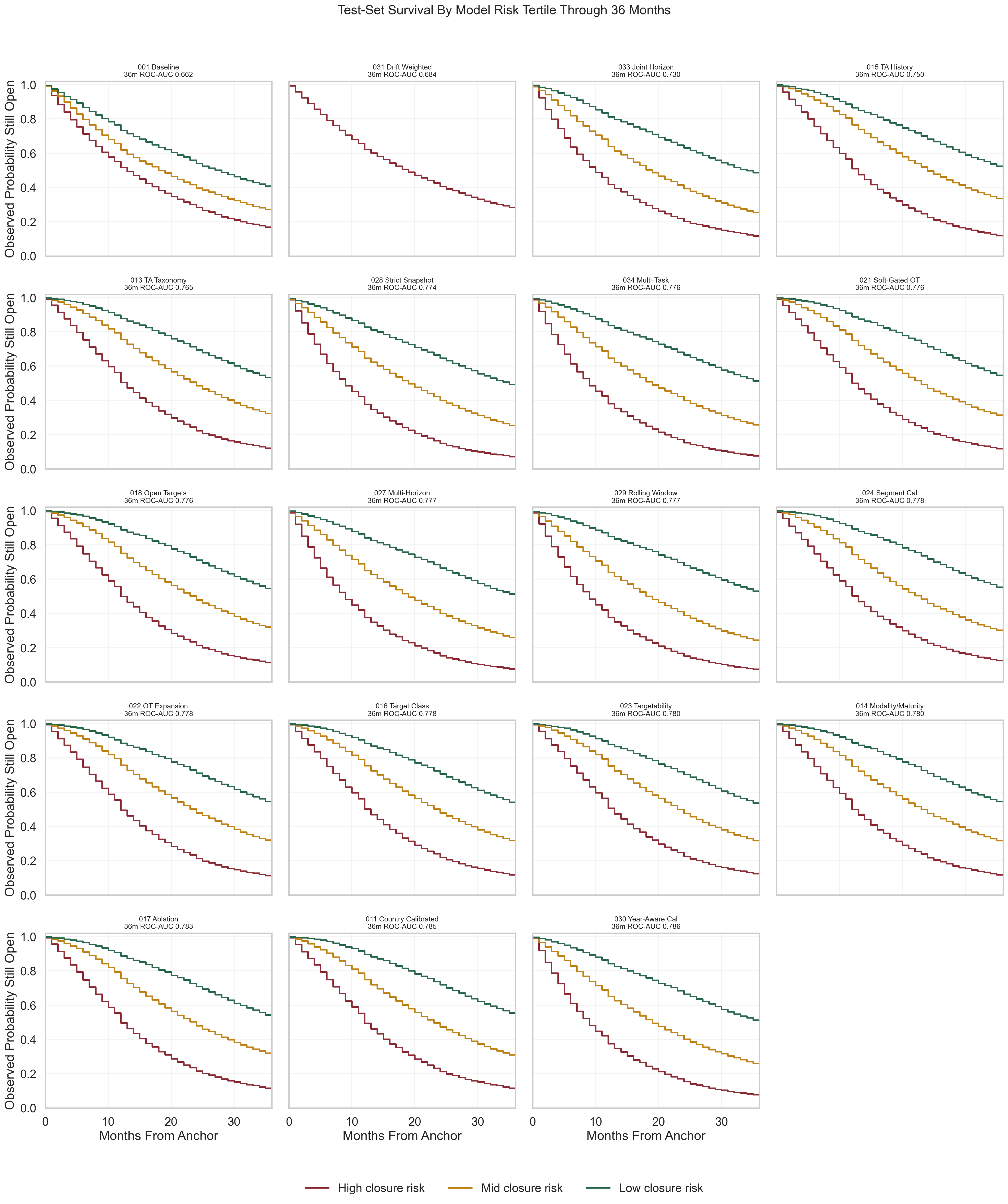
By the time this figure existed, the question was no longer only “which model wins?” It had become about how a whole family of models stratified observed survival on the same test cohort, and how those comparisons changed when the horizon moved out to 36 months.
Example 6: The Focus Shifted Beyond Better Metrics
At some point the project began to saturate. Gains were smaller. New feature ideas were more speculative. That was the right time to stop asking only for improvement and start asking for interpretation.
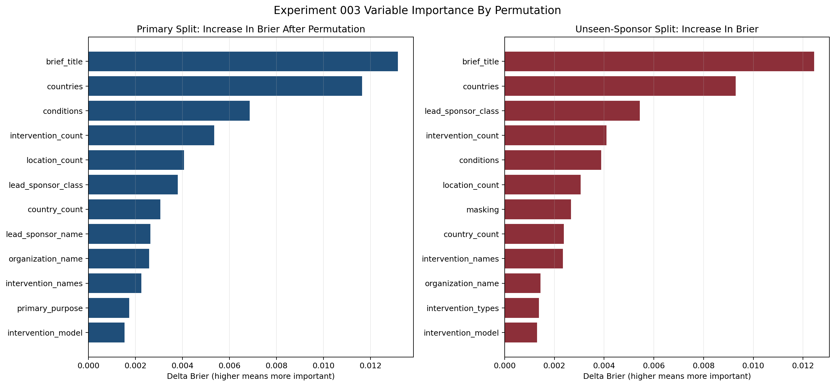
The next question for Sennen was which predictors in the best model were actually actionable in trial design (
/sen:explain). That changed the tone of the work. Sponsor context, intervention identity, and program text were predictive, but not realistically adjustable. Geography footprint, country count, site count, and some design choices were much more actionable.That distinction turned out to be one of the most useful outputs in the whole repo. It moved the conversation from “what does the model use?” to “what could a trial team plausibly change?”
The follow-up question was whether the observed data could support an estimate of how much faster enrollment looked under better settings for those changeable variables. Sennen built an observational speed analysis for that too, while keeping the interpretation explicitly non-causal.
This kind of explanation was the bridge between predictive performance and operational usefulness. It did not magically turn the model into a causal tool, but it made the output much more interpretable for design decisions.
Example 7: There Was No Single Best Model Beyond 12 Months
Later, the metric contract expanded to 24 and 36 months, along with a set of multi-horizon models.
For the original 12-month task, the soft-gated Open Targets model remained the best overall whole-cohort model. But once the horizon moved outward, the ranking changed. Some therapeutic-area-heavy models became more competitive at 24 months. Some rolling-window or horizon-specific approaches looked better at 36 months. A fully pooled multi-horizon model was too blunt, while a partially shared multi-task setup was better, but still not universally best.
That was an important result because it prevented a lazy conclusion. There was no single model that “won everywhere.” The right model depended on the horizon and the metric being optimized.
What This Project Produced
By the end, the project had something more useful than a single benchmark number.
It had:
- a reproducible ingestion and preprocessing pipeline over the full interventional ClinicalTrials.gov corpus
- a leakage-aware temporal and unseen-sponsor evaluation setup
- a strong month-12 launch-time model for registry open-state persistence
- a record of failed branches, not just successful ones
- explanation work that separates predictive context from actionable design levers
- a multi-horizon view showing that model quality depends on the time horizon
Just as important, it had a visible collaboration pattern. The prompts stayed short and directional. Sennen did the heavy lifting: data access, cleaning, experiment implementation, reruns, plots, and comparisons. Then the work was redirected based on what the results showed. That cycle is why the final result is more convincing than a post-hoc tidy story would have been.
What It Still Does Not Do
This is still not a clean model of real-world enrollment speed.
It does not observe site-level accrual directly. It does not establish causal design effects. It does not turn registry metadata into a universal forecast of trial success. And it should not be sold that way.
What it does do is narrower and more defensible: it predicts a registry-derived open-state proxy from launch-time information, under a much more rigorous evaluation setup than the project started with.
The Real Lesson
The main lesson from the project is not to tell the AI “use model X.” It is that a useful applied ML workflow often emerges by tightening the question faster than you escalate the architecture.
The project started with a request for a predictor. Sennen forced a better target definition. It moved on to data, where Sennen surfaced the defects. It moved on to better models, where Sennen showed which ones were not actually better. It ended with the practical question of what could be changed, and Sennen produced importance values that could support a decision workflow.
That is why this project feels educational in retrospect. Not because it found a magic model, but because it kept getting more specific, more reproducible, and more robust.